How to Create Pivot Tables in Excel

Click on the Data menu and choose Pivot Table and PivotChart Report. (Note: in Excel 2007/2010 go to Insert>PivotTable)

Set your options in the prompt as below

Specify the location of the data you are going to summarize. If you have your data in an Excel list that is currently open, Excel will automatically select the cell range. Click "Next."

Ensure the New Worksheet option is selected after you click Next from the previous step. Once you've done that, click "Finish."

If necessary, adjust the range in the Table/Range text box. This is located under the "Select a Table" option button. If the data source for your pivot table is an external database table created with a separate program, such as Access, click the "Use an External Data Source" option button. Click the "Choose Connection" button and then click the name of the connection in the Existing Connections dialog box.

Select the location for the pivot table. Excel's default mode builds the pivot table on a new worksheet it adds to the workbook. To make the pivot table appear on the same worksheet, click the "Existing Worksheet" option button. Indicate the location of the first cell of the new table in the "Location" text box.

Click OK. Excel should add a new blank grid for the pivot table and display a PivotTable Field List task pane. This panel will be divided into two sections.

1)"Choose fields to add to report" list box with the names of all the fields in the source data for the pivot table.
2)An area divided into four drop zones at the bottom: Report Filter, Column Labels, Row Labels and Values.

Assign the fields in the PivotTable Field List task pane to the various parts of the table. Drag a field name from the "Choose fields to add to report" list box into one of the four drop zones.

Manipulate the pivot table as needed until your ideal results appear.

Parts of a Pivot Table

Report filter: This area contains the fields that enable you to page through the data summaries shown in the pivot table by filtering out sets of data. They act as the filters for the report. For example, if you designate the Year field from a table as a Report Filter, you can display data summaries in the pivot table for individual years or for all years represented in the table.

Column labels: This area contains the fields that determine the arrangement of data shown in the columns of the pivot table.

Row labels: This area contains the fields that determine the arrangement of data shown in the rows of the pivot table.

Values: This area contains the fields that determine which data are presented in the cells of the pivot table — they are the values that are summarized in its last column (totaled by default).

Page field: A field from the source data that you assign to a page (or filter) orientation in a Pivot Table report.

Data field. A field from the source data that contains values to be summarized. For example, Sum of Sales is a data field.

Column field: A field from the source data that you assign to a column orientation in a Pivot Table report. For example, Type is a column field.

Item: A subcategory of a row, column, or page field.

Row field: A field from the source data that you assign to a row orientation in a Pivot Table report. For example, Region and Salesperson are row fields.

Data area: The cells in a Pivot Table report that contain summarized data.

How to remove/hide duplicate rows

To Remove duplicate rows:
Select the table containing duplicated rows, click Data on the toolbar-->Click Remove Duplicates
Select the columns to include in identifying duplicates, click OK. This deletes away all the repeated rows

To just Hide duplicate rows
Select the table containing duplicated rows, , click Data on the toolbar-->Filter-->Advanced
Check Unique records Only and Click Ok.

To unhide, just click Clear beside Filter

How to create a drop down list

You need to have a list of values first

For my example I created a separate sheet with just two cells Yes and No

To force a cell to accept only Yes/No, click the cell, click Data on the toolbar and click Data Validation.
On the pop up, choose List from Allow: and choose the two cells containing 'Yes' and 'No' as Source:
See below screen.

Click ok and you are done, you can apply the drop down to other cells as well by copying and pasting.

Note: In older versions Excel 2003 and below, the source of the list (Cells of Yes/No in this case) must be in the same sheet as the drop down, kind of weird.

Humour: Some cells and ranges that you may have heard about

Just for laughs

Some cells and ranges that you may have heard about:

A1	The steak sauce cell
IM21	The legal drinking age cell
K9	The dog cell
AK47	The assault weapon cell
IV2	The second intravenous solution cell
B9	The malignant cell
HI5	The alternate handshake cell
AH:HA	The discovery range
F16	The fighter jet cell
AM:FM	The radio range
ET2	The Brute' cell
AW42	The root beer for two cell
BU:BU	The erroneous range
BY:BY	The farewell range
IC2	The double-vision cell
IQ100	The average intelligence cell
HO:HO	The Santa Claus range
GO2	The destination cell
FU2	The same to you cell
EX2	The second former spouse cell
CU8	The oil-rich country cell
BU10	The shirt fastener cell
BC49:BD1	The '96 Presidential Election results range
AG1:GB1	The '00 disputed Florida vote range
T42	The old soft-shoe cell
U2	The Irish rock group cell
BI123	The Lotus marketing slogan cell
C4	The explosive cell
V8	The vegetable juice cell
R2:D2	The android range
I1:U1	The tied game cell
AP:ES	The Simian range
H8:U2	The ex-wife range
IN2:CA9	The dog-lover range
AC:DC	The electric range
D84:U2	The double date range
I12:CU2	The "when can we meet" cell

How to get classic pivot table view in Excel 2010

For those of you who are used to pivot tables in Excel 2003/2007 like me, these are the steps to get the classic look for pivot tables in Excel 2010. I don't know about you but I still like the familiar look and feel from Excel 2003.


Difference between the new and classic pivot table: The new version group the Row Labels together (I don't usually want that)

Right click ON the pivot table --> PivotTable Options

Click Display tab and check Classic PivotTable layout

We are not done yet, if you want to see merged cells for grouped rows:
Click ON the Pivot table again--> Click Design on tool bar

On PivotTable Styles, click on the bottom down arrow to expand all styles and click Clear
There you have it! Classic pivot table view

How to select table quick

One way is to drag from the upper left corner of the table to the bottom right corner, but what if the table has 60,000 rows?

Don't worry, Ctrl + *

Selects the current region around the active cell, enclosed by blank rows and blank columns.

How to get first day of the month

Using the DATE function

=DATE(YEAR(TODAY()), MONTH(TODAY()), 1)

You can replace TODAY() to get first day of any date

How to use DATE function

The DATE function seems "not so useful" at first sight, enter the year, month, day numbers to get a date. Why would you want to do that in a function when you can just enter the date text directly into the cell, saves time and more human.

Well the DATE function has more uses than you think, it serializes date. Try entering erroneous values into the inputs. For example the 31st day in September, or 13 as month.

I show you what happens if you do that:

=DATE(2011, 9, 31) returns 1 October, 2011

=DATE(2012, 13,4) returns 4 January, 2013

Our first line,  31st Sept 2011 will be serialized to the next day of 30 Sept 2011, since there's only 30 days in Sept, which is 1st Oct 211.

Our second line will be 4th of imaginary month of December plus one 2012, 4th Jan 2013 will be return. The next year date, the next month after Dec will be Jan.

Cool huh? Use your creativity and this DATE function can get you far.

Try getting last day of previous month by using 0 as input for day
=DATE(2012, 13,0) returns 31 December, 2012
=DATE(2012, 12,0) returns 30 November, 2012

Or you just want to get the date after 40000 days later from a date, say 28 Feb 12

=DATE(2012, 2, 28+40000) returns 18 October, 2101

Oh well I will be gone by then and Google might succeed in taking over the world.

Get last day of previous month

=EOMONTH(TODAY(), -1)

Use this function to get last day of previous month from today.


EOMONTH Function is only available for Excel 2007 and above

If EOMONTH function is not available, use this:
=DATE(YEAR(TODAY()), MONTH(TODAY()), 0)

The DATE function will return a date value when you enter in the year, month and day as inputs, what is magical about the DATE function is displayed in my example. I used 0 as the last input for day, this automatically returns the last day of the previous month :)

Get Last day of the month for any date

=EOMONTH(D1,0)

Use this formula to get the last day of the month for the date, D1 is the cell containing the date.

EOMONTH function is only available for Excel 2007 and above, to get last day of the month for older versions of Excel, use this:

=DATE(YEAR(D1),MONTH(D1)+1, 0)

Note:
The DATE function will return a date value when you enter in the year, month and day as inputs, what is magical about the DATE function is displayed in my example. I used 0 as the last input for day, this automatically returns the last day of the previous month,  notice I add one to month? :)

How to display millions as M

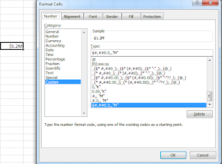
Right click the cell containing the number, choose format cells

Choose Customer as Category, type in #,##0.0,,"M" in the Type: box, click ok

The number of zeros behind the decimal point will decide how much decimal places to show. For example a cell with 1190000 typed in will show 1.2M for #,##0.0,,"M" as custom format.

If you need a dollar sign in front, just use  $#,##0.0,,"M"

How to display thousands as K

Right click the cell containing the number, choose format cells

Choose Customer as Category, type in 0.00,"K" in the Type: box, click ok

The number of zeros behind the decimal point will decide how much decimal places to show. For example a cell with 2519 typed in will show 2.52k for 0.00, "K" as custom format.

If you need a dollar sign in front, just use  $0.00, "K"

How to use Vlookup

 Useful for matching rows between two sets of tables.

Vlookup is good for:

1. Appending columns from this table to that table.
2. Finding missing records.
3. Finding similar records.

Inputs for Vlookup:

1. Lookup_value: The value to search in Table_array
2. Table_array: The set of table to search upon, first column in your selection will be matched with Lookup_value in the search.
3. Col_index_num: Column number in your Table_array to return when a match is found.
4. Range_lookup: I always set to false for an exact match. Try true to return the next largest value that is less than the Lookup_value (You can imagine the funny results involving text lookups when Range lookup is set to true, therefore I always set it to false)

See the example below on getting names from the left table to the right table based on the GuestID

Claire was formulated on I3 with the formula =VLOOKUP(G3, $A$3:$C$6, 2, 0), in human language means search for G3 in Guest table (A3:C6) and return column 2 (Name) of Guest Table if found, use exact matching. To append the name and age to the rest of the rows in Guest Check in Log, just copy and paste from cell I3 and J3, Excel automatically increments the Lookup_Value

IMPORTANT: A common mistake is forgetting to fix the selection of table array when applying vlookup for the whole column by copying and pasting the formula for every row. To prevent that, put $ in front of the column and row labels eg. $A$1:$B$3, just highlight the range and press F4 to do that.

It's best to have an unique column to identify your rows between two sets of data for a good look up. What if an unique identity for a row is not available? What I will do is use the "&" to join some columns together, columns that you feel when combined, forms a unique identity 

See the column Created Identity as an example

That's all! Simple and useful function, good luck finding stuff!